G'MIC
NOISE

noise
noise_hurl
noise_perlin
noise_poissondisk

These are my conclusions based upon experimentation. But then, my conclusions are often wrong... and may well change by the time next we meet. Either way, images follow (and the command line is but a few keystrokes away), so it might be best (as it almost always is) to reach your own conclusions.

• noise
• Pushes full-coverage gaussian-static onto the indicated images.
  • The entire image is covered.
  • The colour tends toward the middle of the range for blank images.
  • For images which start with colour, the colour values shift by a random amount controlled by the first parameter: std_deviation.
• A discussion of the various modes for this command follows the first set of images.
• noise_hurl
• Partial-coverage colour-spectrum static is applied randomly.
• In the images below, there is obvious clumping.
• I believe the colour mode is gaussian.
  • And as such, tends toward the middle of the spectrum.
• I believe the spacial scattering is random.
  • Hence, the clumping.
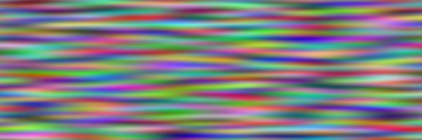
• noise_perlin
• The output is similar to that which turbulence provides.
  • I sort of like turbulence.
• noise_perlin provides linear stretching, though.
  • And that can be cool.
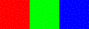
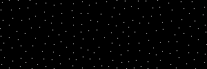
• noise_poissondisk
• I like this pattern the best.
• And it allows for fine-tune control of the spacing.
• But the output is monochromatic
• I will discuss the algorithm used for noise_poissondisk after the section covering the modes available for noise.

Modes

I like G'MIC. I would not be writing this page if I did not. But the documentation leaves a lot to be desired... by me if no one else.

As far as I know, gmic help noise brings up the entirety of the official documentation. Now, I could be wrong. And there might be some wonderful website where the commands are documented in exhausting detail. But I haven't found it. And in fact, sans a picture or two (or several hundred of them, typically one per command), the G'MIC The Handbook is even sparser on the words than that which is available on the command line.

Any-The-Way, entering gmic help noise at the Command Line (Win 10, PowerShell, the serious hobbyist's choice) indicates that noise has two parameters: std_deviation>=0[%] and _noise_type.

The >=0[%] at the end of std_deviation>=0[%] means:

• >=0
• The passed value must be greater than or equal to zero.
• Passing -1 throws an error.
  • I know, as I just tried.
• [%]
• Either an integer or a percent is acceptable.
  • At first glance, this would seem to indicate a choice between Standard Deviation (not something I really understand) and Percents (something that I do).
  • But that's not always the case.

While _noise_type (that is to say the mode) is anybody's guess... until one experiments, of course, which is how I reached the following conclusions.


Um, scratch that. I was being a bit optimistic when I wrote that, as the results of my experimentation are highly unsatisfying.


So, let's start over.

As follows (right after that curly braced indented aside) is my test code.

gmic `
    input '(1,0,0^0,1,0^0,0,1)' `
    normalize 0,255 `
    resize 300,100 `
    +noise[0] 50,2 `
    +noise[0] 50%,2

• gmic
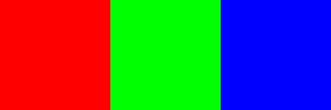
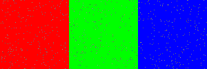
• Calls G'MIC.
• input '(1,0,0^0,1,0^0,0,1)'
• Creates a three pixel wide image, consisting of a Red Pixel, a Green Pixel, and a Blue Pixel.
  • In truth, the Pixels are of value (1,0,0), (0,1,0), and (0,0,1).
  • But because G'MIC is so awesome, it's pretty close to having a Red-Green-Blue image.
• normalize 0,255
• The Colour Space is stretched from 0-1 to 0-255, giving a True RGB Image.
• resize 300,100
• Enlarges the image from 3x1 to 300x100 with no blurring along the boundary.
  • Sweet!
• +noise[0] 50,2
• + adds the resultant image to the stack.
  • No + and the target image is altered in place.
• noise calls the noise command.
• [0] means operate on the first image on the stack.
  • No explicit target and the command is (typically) applied to every image on the stack.
• 50,2 are the passed parameters.
  • 50 is the Standard Deviation.
    • Um, no it's not.
    • Not in this case.
  • 2 is the mode.
    • Yes, in fact, it turns out that it is.
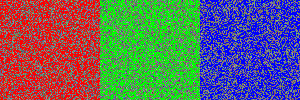
• +noise[0] 50%,2
• The only thing that is different here is the Percent Sign.
• There is no ending output, so G'MIC calls an implicit display.
• display is awesome!
  • If I am going to be honestly negative (cutting, critical, and/or dismissive), then I need to pay honest homage, as well.
  • And display is awesome!

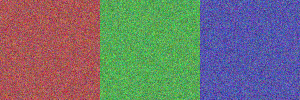
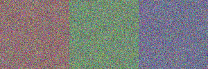
In Display Mode, the preceding code outputs to screen, something like this:

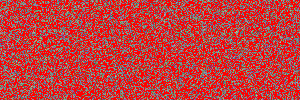
Please note the overwhelming similarity between the second image (the second set of Red, Green, Blue Bands) and the third image. It would appear (to me, if absolutely no one else) that in Mode 2 (Salt & Pepper), there is no difference between 50 and 50%... and in other Modes, there is a great deal of difference.



Mode 0 - Gaussian

I am going to guess (wildly, without any concern whether I am right or wrong or by how incredibly much) that:

If the First Parameter is a Number (not a Percent), a Standard Deviation has been passed. This is beyond my pay grade and/or mathematical ability. But I would surmise that between the Colour Range (0-255 in this case) and a Standard Deviation, one (not I, but someone) can (or could) compute a Random Number via the Gaussian Method (surely, you, if not I, must know what this means).

In short, for each Pixel, a Random Number is thus computed and added to the Pixel's initial value.

While if the First Parameter is a Percentage, for each Pixel, a Random Gaussian Number (seriously, this is so basic, I'm not even going to try and explain it) between -1.0 and +1.0 is computed (a number which hovers about the center, i.e. 0.0) and this number is multiplied by the Range (0-255 in this case, so x255) and added to the Pixel's original value. This step being repeated (with different Random Numbers of the Gaussian sort) for each Pixel.

Too complicated?

Might I recommend sticking with Percents, viewing projects incrementally in the Display Viewer, and trying out different values.

• It's Full Image Coverage.
• Every Pixel will change value.
• The changing values hover about the existing.
• It's a plus or minus to the existing value.
• Any images will need to be re-normalized prior to saving.
• Values can easily exceed 255.
• Negative numbers are possible...
  • Likely, even.
• None of this will be obvious by just looking at the image in the Viewer.
  • Happily, information regarding individual Pixels is easily obtainable in the Viewer.

Mode 1 - Uniform

Wow!

You're still reading.

Just... Wow!

I must admit, I was not expecting that.


Um, The Uniform Mode... er... ah... it selects a Random Number (like at Random) from a Uniform Distribution of Numbers Between -1.0 and +1.0 (so, like, it uses a Uniform Probability Model rather than a Gaussian one)... and from there it's pretty much like Mode 0.

Well, I mean, I could be right.



Mode 2 - Salt & Pepper

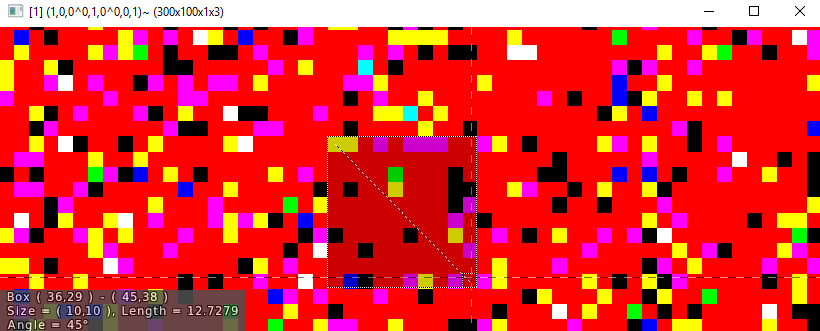
I found no difference between an Integer and a Percent for the first Parameter. For the previous two Modes, Percents typically had a greater effect. However, that was then, this is now. And I can see no difference between 50 and 50% in Salt & Pepper Mode.

The First Parameter seems (well, I am a complete idiot if I am wrong about this, which has often proved to be the case, so really, that says nothing; anyway, it looks to me like) the First Parameter controls the Percent Coverage. It's hard to get more than 100% Coverage. As in, I saw no difference between 100% and 200%. And the Coverage at 25 (or 25%) looked to be at about 25%.

Go Figure!

Oh, wait!

Have I said how awesome the Display Viewer is? I have? OK. Have I mentioned how awesome the Display Viewer is in the last thirteen seconds?

Not including the backwards mention in the preceding paragraph, which doesn't really count, as it was more of a question than a statement?

Huh?

Have I, wise guy?

Eh, I don't know the answer to that convoluted question either.

So, I will say it again, just to be on the safe side.

The Display Viewer is Awesome!

It! Is! Awesome!

But don't let my use of gratuitous exclamation marks sway you. The Viewer can stand on it's own.

Yeah, according to my count that's 25 Off-Colour Pixels in a Random (you'll just have to take my word on it) 10x10 Square. So, the First Parameter clearly (quite clearly, clearly impossible for it to be anything else or for me to be wrong... ever) is the Percentage of Pixels to Change. And this is true whether the number passed is an Integer or a Percent.

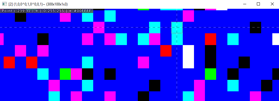
Now, the output of Salt & Pepper is a bit more dynamic. With an All Black Black & White Image, the noise registered as either -1 or 1. In my Tri-Colour Test Image, I got either a 0 or 255 in each of the three Colour Bands. So, like, (255,255,0) was an acceptable bit of noise. While for an actual image, I got what I am going to assume are Random Values between 0 and 255.

Clearly, the input type is important... so, playing around is important. Luckily, the Display Viewer makes this easy. In the image below, I'm hovering over a single Pixel. And the Viewer is telling me all sorts of information about it... including its RGB Colour.

Mode 3 - Poisson

Eh, I am not going to try and discriminate between Poisson, Gaussian, and Uniform. They all seem (keeping in mind that I am nearly blind; and as such, any visual interpretation on my part is not to be trusted, lord knows I do not; but whatever, it looks) to be Full Coverage (like I said, to me): i.e. each Pixel is changed by a varying amount.

One thing nice that I did notice about Poisson was that it did not change Zero Pixels, which I am going to guess means the final step is Multiplication (Existing x Poisson) rather than Additive (Existing + Uniform).

Or in other words, the Poisson Noise that appeared in the Red Bands of my Tri-Colour Test Image were still Red.

Um, yeah.

An example image might be nice here. But it's a sort of boring image, so I will not be inserting it. Instead, I'll suggest running the following and looking at the output to see what I mean when I say the reds stay red.

gmic `
  input '(1,0,0^0,1,0^0,0,1)' `
  normalize 0,255 `
  resize 300,100 `
  +noise[0] 50,3

Mode 4 - Rice

Rice is Full Coverage, as well. And nothing special is standing out (to my razor focused eyesight) to differentiate its output from that of the first two modes.

Poisson Disk

noise_possiondisk accepts two parameters: radius and max_sample_attempts with default values of 8 & 30, respectively. Though, I just seem to throw errors in PowerShell if I don't include any parameters, so I'd fill them in. But then, that's just me, you know, on account of the errors and all.

Anyhow, radius is as it sounds, a radius. And max_sample_attempts is a real solid name for a parameter which limits the number of sample attempts.

And with that bit of nonsense out of the way, I'd say the way noise_possiondisk works is fairly simple... once one knows the secret.

1. A Random Point is selected from The Input Image and put on both The Stack and The Noise Image.
• Since we will pop from The Stack at Random, it's not really a stack.
• The Noise Image is the final output of this algorithm.
  • The Noise Image is laid back on top of The Input Image.
2. From The Stack, an Active Point is Randomly Selected.
• So, like I said, it's not really a stack...
  • More like a list.
• Though, if I were implementing this algorithm (thus, if I were NOT implementing the Poisson Disk Algorithm, but something similar), I'd pop an Active Point from The Stack, examine it 'till exhaustion, and be done with it.
3. For The Active Point, a number of Possible Points equal to max_sample_attempts are randomly computed such that each Possible Point is at least radius distance from The Active Point and no more than 2*radius distance from The Active Point.
4. This list of Possible Points is examined in order.
• If any of these Possible Points is not within radius distance from any other Point already on The Noise Image, place the Possible Point on The Noise Image and return to the second step.
  • The Active Point is NOT popped.
• If not, none of the Possible Points are added to The Noise Image and The Active Point IS popped from The Stack.
5. If there are any Items (call them Points) in The Stack, return to Step 2.
6. Ah, you've reached The End.
• As such, The Stack is empty...
  • Or my explanation contains a cognitive error.
• The Noise Image is the output...
  • Applied Mono-Chromatically.

For noise_possiondisk the output is applied to the input image as a maximum value white dot.

The above image was created by the following code.

gmic `
    input '(1,0,0^0,1,0^0,0,1)' `
    resize 300,100 `
    normalize 0,255 `
    noise_poissondisk 10,20 `
    output save_name.png

Personally, I like the control the algorithm provides.

Goodbye

I thank you for your time.

I thank Robert Bridson for his Algorithm.

And I thank the fine folks at G'MIC for putting together such awesome code.



I tell you what. Rather than begging a beer, why don't we all sit back in our respective abodes, pop the top to the frothy beverage of our choosing (I'll be making mine a Cream Soda), and call it a wash. Or if that doesn't suit you, the next time you feel like hitting somebody, don't.